WSM Decision Support System - The Method

1        Water Availability

The Water Availability Module constitutes the second preprocessor of the WSM Decision Support System aimed at  estimating the amount of water that is available in a water resource system. The water sources considered in the WSM package comprise of surface water, such as artificial or natural lakes and the river network system, and of groundwater, renewable and not.

Water availability modelling generates monthly time series of forecasted available resources for each water source of the system. More specifically, the output of the module concerns natural recharge for renewable groundwater and surface runoff for reservoirs and river reaches. Scenarios can be implemented in two ways, depending upon the type of input data by:

• defining a set of customized years to be repeated in time, based upon real observations at existing monitoring stations, and

• estimating runoff and natural recharge from a surface water balance performed on a monthly time step.

In the first case, calculations are based on monthly average year data of run-off for lakes and river reaches and infiltration for renewable groundwater. User-input can be obtained from statistical analysis of existing, recorded data. Scenarios are formulated through customising a series of base years, where available resources are defined as having monthly positive or negative rates with respect to the normal (average) one.

The alternative (Figure 1) for building availability scenarios is through water balance computations performed at the watershed level. Time series of available runoff and infiltration are computed for selected river reach nodes, lakes and aquifers. User-input is defined as a set of required maps, among which are those of hydro-geological catchments relevant to aquifers and lakes and the Digital Elevation Model (DEM) of the area under study. As far as meteorological data are concerned, twelve maps of precipitation, reference evapotranspiration (ETP) and temperature, containing monthly data for the average year are used as input. There are three ways to build scenarios:

• by repeating the base year as it is for the entire duration of the scenario,

• by defining a total increment over the entire period, either annual or monthly, thus defining a yearly or monthly trend, or 

• through building up a sequence of previously created base years.

Evapotranspiration computations can either be performed using raw data, or through the application of the Thornthwaite formula, taking into account the altitude distribution of the region.

A stochastic option is also available; the idea involves generating a certain number of forecast discharge time series based on a statistical analysis of historical discharge data series. The trend of historical data is kept in the forecast and fluctuations produced try to maintain  the statistics of the historical fluctuations, such as mean value, standard deviation and skewness to the greatest extent.

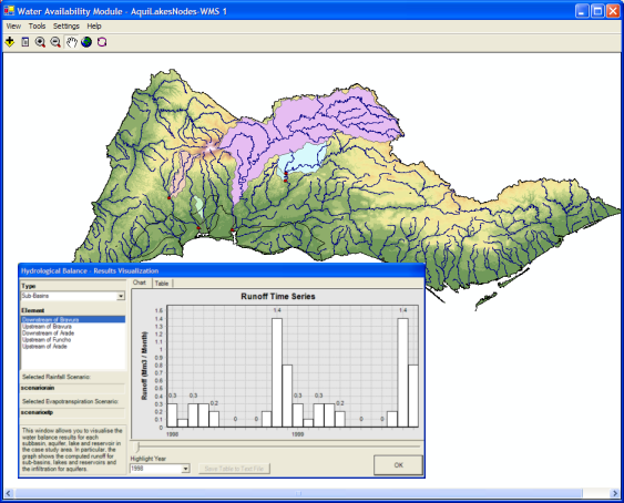
Figure 1. The Water Availability Module of the WSM Decision Support System
(Click here to view an enlarged image of the screenshot)

2         Water Demand

Estimation of water requirements for each use is based on commonly applied models, carefully customised to account for data availability limitations. Irrigation demand is modeled according to the FAO crop coefficient method, incorporating also conveyance, distribution and application efficiencies. Domestic and industrial demands can either be modeled on the basis of different activities, where each is assigned a different level and consumption rate, or through a more simplified approach, i.e. on the basis of population variations and consumption rates.

Scenarios are generated by specifying appropriate growth rates to the key variables (Drivers) that govern the water demand of the uses, such as population for domestic use, cultivable area and livestock for agricultural practices, production growth and energy requirements for industries and hydropower plants respectively. This specification can be made in two ways, either globally for all uses and requirements, or by assigning specific demand expressions for each use. The parameters that can be used for the formulation of alternative scenarios are summarised in Table 1.

Table 1. Attributes for building demand scenarios

3         Water Allocation

Water allocation is the heart of the developed Decision Support System, on which the forecasting of the state of the system, under different scenario assumptions and application of instruments, is based.

Several methodologies have been used increasingly  over the last decades for the optimal design, planning, and operation of water resource systems. The two basic categories of water resource models are simulation and optimisation models (Wardlaw,1999). Mays (1996) carried out a wide review of these models. Some authors (Mannochi and Mecarelli, 1994; Reca et al., 2001) introduced economic objective functions in irrigation water allocation models. However, the development of economic objective functions still remains closely related to the specific characteristics of the area for the application of the model, making most of the developed models not readily adaptable to a case study area.

In the WSM DSS, water allocation is achieved through a simulation model, aiming to minimize water shortage under limited water supplies. In situations of water shortage, a conflict arises in how to distribute the water available from the various supply sources to uses connected to them. The model can solve this problem using two user-defined priority rules.

First, competing demand sites are treated according to their assigned priorities. Each demand site is characterized by a priority, which can express social preference or constraints (e.g. urban water needs would be met first), economic preference (highest priority is given to activities with the highest economic value), developmental priorities of a particular economic sector, or a system of water rights. In case that a particular use can be supplied by more than one resource, supply priorities are used to rank the choices for obtaining water. Supply priorities can express: (a) cost preference for supply paths with low costs (b) quality preference of uses (e.g. domestic or industrial use) for supply sources with high water quality; (c) need for the protection of resources and the creation of strategic reserves which is modelled through the assignment of very low priorities.

The mathematical concept of the model is to find stationary solutions for each monthly time step. For each month the problem is to find on the network the flow, that minimizes the water shortage on all uses and requirements, subject to constraints related to the capacity of supply links, estimated demand and available supplies. The model formulated is reduced to an equivalent maxflow problem, which is solved using the Ford-Fulkerson method, known as the Augmenting-Path Maxflow algorithm (Dolam and Aldous, 1993; Sedgewick, 2002).

4         Modelling of alternative actions - Strategy Formulation

A characteristic of the DSS is that it predefines a number of “abstract” water management instruments (actions) and incorporates them as methods into the system. Those methods modify the properties of the network objects accordingly or introduce new ones, related to water infrastructure development. An “abstract” action becomes “application specific” by the user-definition of its magnitude, time horizon and geographic domain. An initial set of actions that can be taken into consideration is presented in Table 2.

Actions incorporated are mainly focused on instruments to deal with the frequent water shortages occurring in arid regions. The main aim is to either enhance supply, promoting the protection of vulnerable resources through structural interventions, or to regulate demand through the promotion of conservation measures, technological adjustments for promoting efficiency of water use, and pricing incentives.

Table 2. Summary Table of Policy Options and related Actions incorporated in the WSM DSS

5   Economic Analysis

The primary aim of the economic analysis performed by the DSS is the estimation, according to the results of the allocation algorithm, of financial, environmental, and resource costs. Those costs should be recovered through appropriate water pricing policies from the demand uses (nodes) in order to reach the full cost recovery of water services (WATECO, 2003).

Estimation of financial costs associated with the provision of water supply is rather straightforward, depending on the depreciation of capital construction costs and specific energy and operation and maintenance costs associated with each part of the infrastructure used by each demand use. Two types of environmental costs have been incorporated in the DSS, one for the abstraction and consumptive use of freshwater resources (surface and groundwater) and one for the pollution generation from demand activities.

Resource costs associated with freshwater resources are associated with the scarcity rent of the resource. Scarcity rent is defined as a surplus, the difference between the opportunity cost of water and the per unit direct costs (such as extraction, treatment, environmental and conveyance) of turning that natural resource into product (agricultural crops for farmers, water services for the residence of an urban centre, industrial production etc).

6         Evaluation of alternative water management schemes

Evaluation of alternative schemes is based on a multi-criteria approach that takes into account the entire simulation horizon. In a first step, time series of indicators are computed, describing the behavior of the water system in terms of environmental, efficiency, and economic objectives (Table 3), with the ultimate goal of assisting decision makers in the selection of water management instruments that meet the goals of Integrated Water Resources Management.

Table 3. Indicators used in the WSM DSS evaluation procedure.

The comparison is performed through a multi-criteria analysis based on the computation of statistical criteria for reliability, resilience and vulnerability (Bogardi and Verhoef, 1995; ASCE, 1998). The statistical criteria express the behavior of the monthly or yearly time series of each indicator with respect to the predefined range of satisfactory values that the indicator can assume. Reliability is defined as the probability that any particular indicator value will be within the range of values considered satisfactory. Resilience describes the speed of recovery from an unsatisfactory condition. Vulnerability statistical criteria measure the extent and the duration of unsatisfactory values. Performance for each indicator is computed as the product of the above criteria, and the relative sustainability index of each WMS is estimated as the weighted sum of the performance of the selected indicators.

The output of the evaluation module permits the ranking of alternative water management schemes, and the selection of those most appropriate for dealing with the water management issues faced by the region under study. The module permits comparison of the effectiveness of one or a set of options under different conditions, as well as the inter-comparison between them, in order to select the most appropriate management approaches.

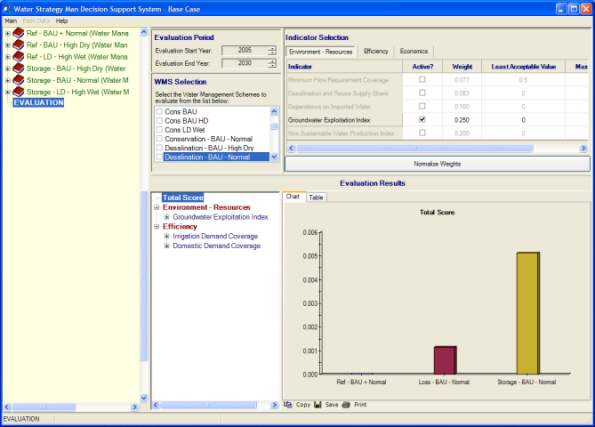
Figure 2. The Evaluation output of the WSM DSS
(Click here to view an enlarged image of the screenshot)

Related References

• Bogardi J.J., Verhoef A. (1995), Reliability Analysis of Reservoir Operation, New Uncertainty Concepts in Hydrology and Water Resources, Cambridge University Press.

• Dolam, A. and Aldous, J. (1993) Networks and Algorithms: An Introductory Approach, Wiley.

• McKinney, D.C, Cai, X, Rosegrant, M.W., Ringler, C. and Scott C.A. (1999), Modelling Water Resources Management at the Basin Level: Review and Future Directions, International Water Management Institute, SWIM Paper 6.

• Mannochi, F., Mecarelli, P. (1994), Optimization Analysis of Deficit Irrigation Systems, J. Irrig. Drain. Eng., 120 (3), 484-503.

• Reca, J., Roldan, J., Alcaide, M., Lopez, R. and Camacho, E. (2001), Optimisation Model for Water Allocation in Deficit Irrigation Systems I. Description of the Model, Agricultural Water Management, 48, 103-116.

• Sedgewick, R (2002) Algorithms in C++ Part 5: Graph Algorithms, Addison Wesley Longman.

• Task Committee on Sustainability Criteria, Water Resources Planning and Management Division, ASCE and Working Group of UNESCO/IHP IV Project M-4.3 (1998), Sustainability Criteria for Water Resource Systems, ASCE Publications, Virginia.

• Wardlaw R. (1999), Computer Optimisation for Better Water Allocation, Agricultural Water Management, 40, 65-70.

• WATECO (2002), Economics and the Environment – The implementation challenge of the Water Framework Directive, A guidance document, European Commission.